Mie Basics

Scott Prahl

April 2021

If miepython is not installed, uncomment the following cell (i.e., delete the #) and run (shift-enter)

#!pip install --user miepython

import numpy as np
import matplotlib.pyplot as plt

try:
    import miepython

except ModuleNotFoundError:
    print('miepython not installed. To install, uncomment and run the cell above.')
    print('Once installation is successful, rerun this cell again.')

Index of Refraction and Size Parameter

When a monochromatic plane wave is incident on a sphere, it scatters and absorbs light depending on the properties of the light and sphere. If the sphere is in a vacuum, then the complex index of refraction of the sphere is

\[m_\mathrm{vac}= m_\mathrm{re}- j\,m_\mathrm{im}\]

The factor \(m_\mathrm{im}=\kappa\) is the index of absorption or the index of attenuation.

The non-dimensional sphere size parameter for a sphere in a vacuum is

\[x_\mathrm{vac} = \frac{2\pi r }{\lambda_\mathrm{vac}}\]

where \(r\) is the radius of the sphere and \(\lambda_\mathrm{vac}\) is the wavelength of the light in a vacuum.

If the sphere is in a non-absorbing environment with real index \(n_\mathrm{env}\) then the Mie scattering formulas can still be used, but the index of refraction of the sphere is now

\[m= \frac{m_\mathrm{re}- j\,m_\mathrm{im}}{ n_\mathrm{env}}\]

The wavelength in the sphere size parameter should be the wavelength of the plane wave in the environment, thus

\[x = \frac{2\pi r } {\lambda_\mathrm{vac}/n_\mathrm{env}}\]

Sign Convention

The sign of the imaginary part of the index of refraction in miepython is assumed negative (as shown above). This convention is standard for atmospheric science and follows that of van de Hulst.

Absorption Coefficient

The imaginary part of the refractive index is a non-dimensional representation of light absorption. This can be seen by writing out the equation for a monochromatic, planar electric field

\[\mathcal{E}(z,t) = \mathcal{E}_0 e^{j (k z - \omega t)}\]

where \(k\) is the complex wavenumber

\[k=k_\mathrm{re}-k_\mathrm{im}=2\pi {{m_\mathrm{re}}\over{\lambda_\mathrm{vac}}}-2\pi j \frac{m_\mathrm{im}}{\lambda_\mathrm{vac}}\]

Thus

\[\mathcal{E}(z,t) = \mathcal{E}_0 e^{-k_\mathrm{im}z}e^{j (k_\mathrm{re} z - \omega t)}\]

and the corresponding time-averaged irradiance \(E(z)\)

\[E(z) = {1\over2} c\epsilon |\mathcal{E}|^2 = E_0 \exp(-2k_\mathrm{im}z) = E_0 \exp(-\mu_a z)\]

and therefore

\[\mu_a = 2k_\mathrm{im} = 4\pi\cdot \frac{ m_\mathrm{im}}{ \lambda_\mathrm{vac}}\]

Thus the imaginary part of the index of refraction is basically just the absorption coefficient measured in wavelengths.

miepython.mie_S1_S2(1.507-0.002j , 0.7086 , np.array([-1.0],dtype=float))

[array([0.02452301+0.29539154j]), array([-0.02452301-0.29539154j])]

miepython.mie_S1_S2(1.507-0.002j , 0.7086 , -1)

((0.02452300864212876+0.29539154027629805j),
 (-0.02452300864212876-0.29539154027629805j))

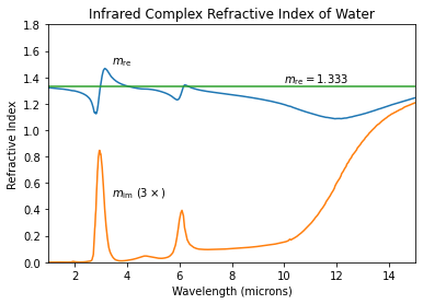
Complex Refractive Index of Water

Let’s import and plot some data from the M.S. Thesis of D. Segelstein, “The Complex Refractive Index of Water”, University of Missouri–Kansas City, (1981) to get some sense the complex index of refraction. The imaginary part shows absorption peaks at 3 and 6 microns, as well as the broad peak starting at 10 microns.

#import the Segelstein data
h2o = np.genfromtxt('http://omlc.org/spectra/water/data/segelstein81_index.txt', delimiter='\t', skip_header=4)
h2o_lam = h2o[:,0]
h2o_mre = h2o[:,1]
h2o_mim = h2o[:,2]

#plot it
plt.plot(h2o_lam,h2o_mre)
plt.plot(h2o_lam,h2o_mim*3)
plt.plot((1,15),(1.333,1.333))
plt.xlim((1,15))
plt.ylim((0,1.8))
plt.xlabel('Wavelength (microns)')
plt.ylabel('Refractive Index')
plt.annotate(r'$m_\mathrm{re}$', xy=(3.4,1.5))
plt.annotate(r'$m_\mathrm{im}\,\,(3\times)$', xy=(3.4,0.5))
plt.annotate(r'$m_\mathrm{re}=1.333$', xy=(10,1.36))

plt.title('Infrared Complex Refractive Index of Water')

plt.show()

# import the Johnson and Christy data for gold
try:
    au = np.genfromtxt('https://refractiveindex.info/tmp/data/main/Au/Johnson.txt', delimiter='\t')
except OSError:
    # try again
    au = np.genfromtxt('https://refractiveindex.info/tmp/data/main/Au/Johnson.txt', delimiter='\t')

# data is stacked so need to rearrange
N = len(au)//2
au_lam = au[1:N,0]
au_mre = au[1:N,1]
au_mim = au[N+1:,1]

plt.scatter(au_lam,au_mre,s=1,color='blue')
plt.scatter(au_lam,au_mim,s=1,color='red')
plt.xlim((0.2,2))
plt.xlabel('Wavelength (microns)')
plt.ylabel('Refractive Index')
plt.annotate(r'$m_\mathrm{re}$', xy=(1.0,0.5),color='blue')
plt.annotate(r'$m_\mathrm{im}$', xy=(1.0,8),color='red')

plt.title('Complex Refractive Index of Gold')

plt.show()

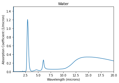
The Absorption Coefficient of Water

mua = 4*np.pi* h2o_mim/h2o_lam

plt.plot(h2o_lam,mua)
plt.xlim((0.1,20))
plt.ylim((0,1.5))
plt.xlabel('Wavelength (microns)')
plt.ylabel('Absorption Coefficient (1/micron)')

plt.title('Water')

plt.show()

Size Parameters

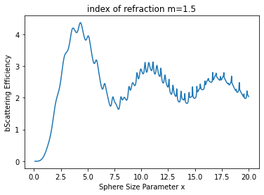
Size Parameter \(x\)

The sphere size relative to the wavelength is called the size parameter \(x\)

\[ \begin{align}\begin{aligned} x = 2\pi {r/\lambda}\\where :math:`r` is the radius of the sphere.\end{aligned}\end{align} \]

N=500
m=1.5
x = np.linspace(0.1,20,N)  # also in microns

qext, qsca, qback, g = miepython.mie(m,x)

plt.plot(x,qsca)
plt.xlabel("Sphere Size Parameter x")
plt.ylabel("bScattering Efficiency")
plt.title("index of refraction m=1.5")
plt.show()

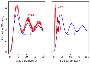
Size Parameter \(\rho\)

The value \(\rho\) is also sometimes used to facilitate comparisons for spheres with different indicies of refraction

\[ \begin{align}\begin{aligned} \rho = 2x(m-1)\\Note that when :math:`m=1.5` and therefore :math:`\rho=x`.\end{aligned}\end{align} \]

As can be seen in the graph below, the scattering for spheres with different indicies of refraction pretty similar when plotted against \(\rho\), but no so obvious when plotted against \(x\)

N=500
m=1.5
rho = np.linspace(0.1,20,N)  # also in microns

m = 1.5
x15 = rho/2/(m-1)
qext, sca15, qback, g = miepython.mie(m,x15)

m = 1.1
x11 = rho/2/(m-1)
qext, sca11, qback, g = miepython.mie(m,x11)

f, (ax1, ax2) = plt.subplots(1, 2, sharey=True)

ax1.plot(rho,sca11,color='blue')
ax1.plot(rho,sca15,color='red')
ax1.set_xlabel(r"Size parameter $\rho$")
ax1.set_ylabel("Scattering Efficiency")
ax1.annotate('m=1.5', xy=(10,3.3), color='red')
ax1.annotate('m=1.1', xy=(8,1.5), color='blue')

ax2.plot(x11,sca11,color='blue')
ax2.plot(x15,sca15,color='red')
ax2.set_xlabel(r"Size parameter $x$")
ax2.annotate('m=1.5', xy=(5,4), color='red')
ax2.annotate('m=1.1', xy=(40,1.5), color='blue')

plt.show()

Embedded spheres

The short answer is that everything just scales.

Specifically, divide the index of the sphere \(m\) by the index of the surrounding material to get a relative index \(m'\)

\[m' =\frac{m}{n_\mathrm{surroundings}}\]

The wavelength in the surrounding medium \(\lambda'\) is also altered

\[\lambda' = \frac{\lambda_\mathrm{vacuum}}{n_\mathrm{surroundings}}\]

Thus, the relative size parameter \(x'\) becomes

\[x' = \frac{2 \pi r} {\lambda'}= \frac{2 \pi r n_\mathrm{surroundings}}{ \lambda_\mathrm{vacuum}}\]

Scattering calculations for an embedded sphere uses \(m'\) and \(x'\) instead of \(m\) and \(x\).

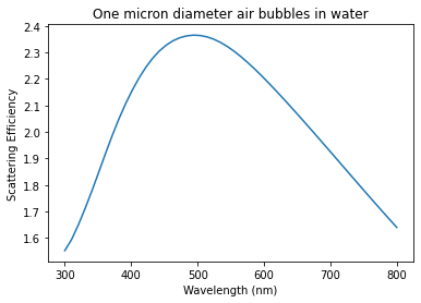
If the spheres are air (\(m=1\)) bubbles in water (\(m=4/3\)), then the relative index of refraction will be about

\[m' = m/n_\mathrm{water} \approx 1.0/(4/3) = 3/4 = 0.75\]

N=500
m=1.0
r=500                            # nm
lambdaa = np.linspace(300,800,N)  # also in nm

mwater = 4/3   # rough approximation
mm = m/mwater
xx = 2*np.pi*r*mwater/lambdaa

qext, qsca, qback, g = miepython.mie(mm,xx)

plt.plot(lambdaa,qsca)
plt.xlabel("Wavelength (nm)")
plt.ylabel("Scattering Efficiency")
plt.title("One micron diameter air bubbles in water")
plt.show()

or just use ez_mie(m, d, lambda0, n_env)

m_sphere = 1.0
n_water  = 4/3
d = 1000                        # nm
lambda0 = np.linspace(300,800)  # nm

qext, qsca, qback, g = miepython.ez_mie(m_sphere, d, lambda0, n_water)

plt.plot(lambda0,qsca)
plt.xlabel("Wavelength (nm)")
plt.ylabel("Scattering Efficiency")
plt.title("One micron diameter air bubbles in water")
plt.show()

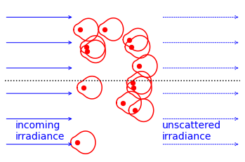
Multiple scatterers

This will eventually turn into a description of the scattering coefficient.

m = 1.5
x = np.pi/3
theta = np.linspace(-180,180,1800)
mu = np.cos(theta/180*np.pi)
s1,s2 = miepython.mie_S1_S2(m,x,mu)
scat = 5*(abs(s1)**2+abs(s2)**2)/2  #unpolarized scattered light

N=13
xx = 3.5 * np.random.rand(N, 1) - 1.5
yy = 5 * np.random.rand(N, 1) - 2.5

plt.scatter(xx,yy,s=40,color='red')
for i in range(N):
    plt.plot(scat*np.cos(theta/180*np.pi)+xx[i],scat*np.sin(theta/180*np.pi)+yy[i],color='red')

plt.plot([-5,7],[0,0],':k')

plt.annotate('incoming\nirradiance', xy=(-4.5,-2.3),ha='left',color='blue',fontsize=14)
for i in range(6):
    y0 = i -2.5
    plt.annotate('',xy=(-1.5,y0),xytext=(-5,y0),arrowprops=dict(arrowstyle="->",color='blue'))

plt.annotate('unscattered\nirradiance', xy=(3,-2.3),ha='left',color='blue',fontsize=14)
for i in range(6):
    y0 = i -2.5
    plt.annotate('',xy=(7,y0),xytext=(3,y0),arrowprops=dict(arrowstyle="->",color='blue',ls=':'))

#plt.annotate('scattered\nspherical\nwave', xy=(0,1.5),ha='left',color='red',fontsize=16)
#plt.annotate('',xy=(2.5,2.5),xytext=(0,0),arrowprops=dict(arrowstyle="->",color='red'))
#plt.annotate(r'$\theta$',xy=(2,0.7),color='red',fontsize=14)
#plt.annotate('',xy=(2,2),xytext=(2.7,0),arrowprops=dict(connectionstyle="arc3,rad=0.2", arrowstyle="<->",color='red'))

plt.xlim(-5,7)
plt.ylim(-3,3)
plt.axis('off')
plt.show()