Mie Scattering Function
Scott Prahl
May 2024
Mie scattering describes the special case of the interaction of light passing through a non-absorbing medium with a single embedded spherical object. The sphere itself can be non-absorbing, moderately absorbing, or perfectly absorbing.
[1]:
import numpy as np
import matplotlib.pyplot as plt
import miepython

%config InlineBackend.figure_format = 'retina'
[7]:
help(miepython.mie)
Help on function mie in module miepython.miepython:

mie(m, x)
    Calculate the efficiencies for a sphere where m or x may be arrays.

    Args:
        m: the complex index of refraction of the sphere
        x: the size parameter of the sphere

    Returns:
        qext: the total extinction efficiency
        qsca: the scattering efficiency
        qback: the backscatter efficiency
        g: the average cosine of the scattering phase function
Goals for this notebook:
show how to plot the phase function
explain the units for the scattering phase function
show a few examples from classic Mie texts
Geometry
Specifically, the scattering function \(p(\theta_i,\phi_i,\theta_o,\phi_o)\) describes the amount of light scattered by a particle for light incident at an angle \((\theta_i,\phi_i)\) and exiting the particle (in the far field) at an angle \((\theta_o,\phi_o)\). For simplicity, the scattering function is often assumed to be rotationally symmetric (it is, obviously, for spherical scatterers) and that the angle that the light is scattered into only depends the \(\theta=\theta_o-\theta_i\). In this case, the scattering function can be written as \(p(\theta)\). Finally, the angle is often replaced by \(\mu=\cos\theta\) and therefore the phase function becomes just \(p(\mu)\).
The figure below shows the basic idea. An incoming monochromatic plane wave hits a sphere and produces in the far field two separate monochromatic waves — a slightly attenuated unscattered planar wave and an outgoing spherical wave.
Obviously. the scattered light will be cylindrically symmetric about the ray passing through the center of the sphere.
[2]:
fs = 10 # fontsize
t = np.linspace(0,2*np.pi,100)
xx = np.cos(t)
yy = np.sin(t)

plt.figure(figsize=(8,4.5))
plt.gca().set_aspect('equal')
plt.plot(xx,yy, color='green')
plt.axhline(0, color='black', lw=0.5)

plt.annotate('incoming irradiance', xy=(-4.5,-2.3),ha='left',color='blue',fontsize=fs)
for i in range(6):
    y0 = i -2.5
    plt.annotate('',xy=(-1.5,y0),xytext=(-5,y0),arrowprops=dict(arrowstyle="->",color='blue'))

plt.annotate('unscattered irradiance', xy=(3,-2.3),ha='left',color='blue',fontsize=fs)
for i in range(6):
    y0 = i -2.5
    plt.annotate('',xy=(7,y0),xytext=(3,y0),arrowprops=dict(arrowstyle="->",color='blue',ls=':'))

#plt.text(0, 1.5, 'scattered\nspherical\nwave', ha='left', color='red', fontsize=fs)
plt.annotate('',xy=(2.5,2.5),xytext=(0,0),arrowprops=dict(arrowstyle="->",color='black', lw=0.5))
plt.annotate(r'$\theta$',xy=(2,0.7),color='red',fontsize=fs)
plt.annotate('',xy=(2,2),xytext=(2.7,0),arrowprops=dict(connectionstyle="arc3,rad=0.2", arrowstyle="<->",color='red'))
plt.text(0,-0.4,'$m_{re}-j m_{im}$',ha='center', color='green',fontsize=fs)
plt.text(1,-1.8,'$n_{environment}$',ha='center',color='blue',fontsize=fs)
plt.xlim(-5,7)
plt.ylim(-3,3)
plt.axis('off')
#plt.savefig('mie-diagram1.png', dpi=300, transparent=True)
#plt.savefig('mie-diagram1.svg')
plt.show()

Scattered Wave
[3]:
fs = 10 # fontsize
plt.figure(figsize=(8,4.5))
plt.gca().set_aspect('equal')

m = 1.5
x = np.pi/3
theta = np.linspace(-180,180,180)
theta_r = np.radians(theta)

mu = np.cos(theta_r)
scat = 15 * miepython.i_unpolarized(m,x,mu)

plt.plot(scat*np.cos(theta/180*np.pi),scat*np.sin(theta/180*np.pi), color='red')
for i in range(12):
    ii = i*15
    xx = scat[ii]*np.cos(theta_r[ii])
    yy = scat[ii]*np.sin(theta_r[ii])
#    print(xx,yy)
    plt.annotate('',xy=(xx,yy),xytext=(0,0),arrowprops=dict(arrowstyle="->",color='black'))


plt.annotate('incident irradiance', xy=(-4.5,-2.3),ha='left',color='blue',fontsize=fs)
for i in range(6):
    y0 = i -2.5
    plt.annotate('',xy=(-1.5,y0),xytext=(-5,y0),arrowprops=dict(arrowstyle="->",color='blue'))

plt.annotate('unscattered irradiance', xy=(3,-2.3),ha='left',color='blue',fontsize=fs)
for i in range(6):
    y0 = i -2.5
    plt.annotate('',xy=(7,y0),xytext=(3,y0),arrowprops=dict(arrowstyle="->",color='blue',ls=':'))

plt.annotate('scattered\nspherical wave', xy=(1,1.5), ha='center', color='red', fontsize=fs)
plt.plot([0],[0], 'ok', markersize=10)

plt.xlim(-5,7)
plt.ylim(-3,3)
plt.axis('off')
#plt.savefig('mie-diagram2.png', dpi=300, transparent=True)
#plt.savefig('mie-diagram2.svg')

plt.show()

Normalization of the scattered light
By default the scattering function is normalized so that the integral over all angles will be the single scattering albedo.
So the scattering function or phase function has at least three reasonable normalizations that involve integrating over all \(4\pi\) steradians. Below \(d\Omega=\sin\theta d\theta\,d\phi\) is a differential solid angle
See https://miepython.readthedocs.io/en/latest/03a_normalization.html for details about other normalization options.
Examples
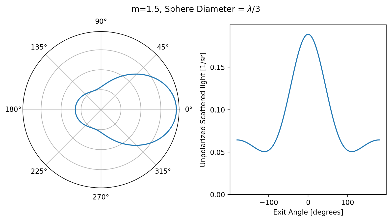
Unpolarized Scattering Function
If unpolarized light hits the sphere, then there are no polarization effects to worry about. It is pretty easy to generate a plot to show how scattering changes with angle.
[4]:
m = 1.5
x = np.pi/3
theta = np.linspace(-180, 180, 180)
mu = np.cos(theta / 180 * np.pi)
scat = miepython.i_unpolarized(m, x, mu)

plt.figure(figsize=(8, 4.5))
plt.suptitle(r"m=1.5, Sphere Diameter = $\lambda$/3")

#fig, ax = plt.subplots(subplot_kw={'projection': 'polar'})
plt.subplot(121, projection='polar')
plt.plot(np.radians(theta), scat)
plt.gca().set_rticks([0.05, 0.1, 0.15])
plt.gca().set_yticklabels([])  # omit radial labels

# Cartesian plot
plt.subplot(122)
plt.plot(theta, scat)
plt.xlabel('Exit Angle [degrees]')
plt.ylabel('Unpolarized Scattered light [1/sr]')
plt.yticks([0,0.05,0.1,0.15])
plt.ylim(0.00, 0.2)

plt.tight_layout()
plt.show()
A similar calculation but using ez_intensities()
[5]:
m = 1.33
lambda0 = 632.8 # nm
d = 200        # nm

theta = np.linspace(-180,180,180)
mu = np.cos(theta/180*np.pi)

Ipar, Iper = miepython.ez_intensities(m, d, lambda0, mu)

plt.figure(figsize=(8, 4.5))
plt.suptitle(r"m=%.2f, Sphere Diameter = %.0fnm, $\lambda$=%.1f nm" % (m, d, lambda0))

plt.subplot(121, projection='polar')
plt.plot(np.radians(theta), Ipar, color='blue')
plt.text(0.3, 0.12, r'$I_\parallel$', fontsize=12, color='blue')
plt.plot(np.radians(theta), Iper, color='red')
plt.text(1.5, 0.10, r'$I_\perp$', fontsize=12, color='red')
plt.gca().set_rticks([0.05, 0.1, 0.15, 0.20])
plt.gca().set_yticklabels([])
plt.gca().set_xticklabels([])

plt.subplot(122)
plt.plot(theta, Ipar, color='blue')
plt.text(40, 0.12, r'$I_\parallel$', fontsize=12, color='blue')
plt.plot(theta, Iper, color='red')
plt.text(55, 0.15, r'$I_\perp$', fontsize=12, color='red')

plt.xlabel('Exit Angle [degrees]')
plt.ylabel('Scattered light [1/sr]')
plt.ylim(0.00,0.2)

plt.tight_layout()
plt.show()

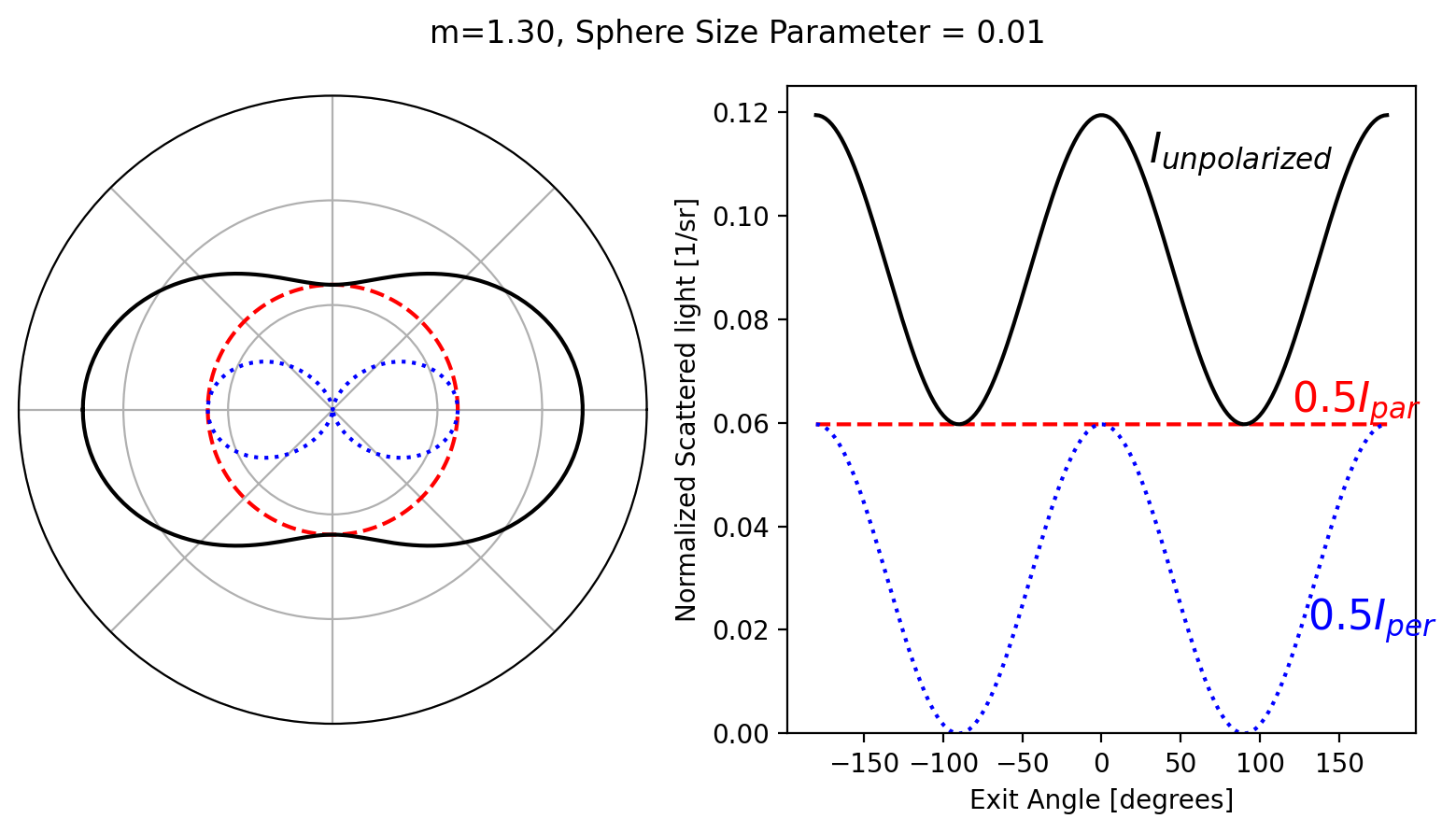
Rayleigh Scattering
[6]:
m = 1.3
x = 0.01
theta = np.linspace(-180,180,180)
mu = np.cos(theta/180*np.pi)
ipar = miepython.i_par(m,x,mu)/2
iper = miepython.i_per(m,x,mu)/2
iun  = miepython.i_unpolarized(m,x,mu)

plt.figure(figsize=(8, 4.5))
plt.suptitle('m=%.2f, Sphere Size Parameter = %.2f' %(m,x))

plt.subplot(121, projection='polar')

plt.subplot(121, projection='polar')
plt.plot(theta/180*np.pi, iper, 'r--')
plt.plot(theta/180*np.pi, ipar, 'b:')
plt.plot(theta/180*np.pi, iun, 'k')

plt.gca().set_rticks([0.05, 0.1,0.15])
plt.gca().set_yticklabels([])
plt.gca().set_xticklabels([])

#plt.title('m=%.2f, Sphere Parameter = %.2f' %(m,x))

plt.subplot(122)
plt.plot(theta,iper,'r--')
plt.plot(theta,ipar,'b:')
plt.plot(theta,iun,'k')

plt.xlabel('Exit Angle [degrees]')
plt.ylabel('Normalized Scattered light [1/sr]')
plt.ylim(0.00,0.125)
plt.text(130,0.02,r"$0.5I_{per}$",color="blue", fontsize=16)
plt.text(120,0.062,r"$0.5I_{par}$",color="red", fontsize=16)
plt.text(30,0.11,r"$I_{unpolarized}$",color="black", fontsize=16)

plt.tight_layout()

plt.show()
[ ]: