Mie Basics
Scott Prahl
January 2025
[1]:
%config InlineBackend.figure_format = 'retina'

import os
import sys
import numpy as np
import matplotlib.pyplot as plt
import importlib.resources

if sys.platform == "emscripten":
    import piplite

    await piplite.install("miepython", deps=False)
    os.environ["MIEPYTHON_USE_JIT"] = "0"  # jupyterlite cannot use numba

import miepython as mie
Index of Refraction and Size Parameter
When a monochromatic plane wave is incident on a sphere, it scatters and absorbs light depending on the properties of the light and sphere. If the sphere is in a vacuum, then the complex index of refraction of the sphere is
The factor \(m_\mathrm{im}\) is the index of absorption or the index of attenuation.
The dimensionless sphere size parameter for a sphere of radius \(a\) is
where \(\lambda_\mathrm{vac}\) is the wavelength of the light in a vacuum.
If the sphere is in a non-absorbing environment with real index \(n_\mathrm{env}\) then the Mie scattering formulas can still be used, but the index of refraction of the sphere becomes
The dimensionless size parameter for a sphere includes the wavelength. This should be the wavelength of the plane wave in the environment, thus
Sign Convention
The sign of the imaginary part of the index of refraction in miepython is assumed negative (as shown above). This convention is standard for atmospheric science and follows that of van de Hulst.
Starting in version 3.0.0, miepython silently converts positive imaginary index of refraction values to negative ones. This may or may not be a good thing.
Field Conventions (Near-Field)
For miepython.field, the electromagnetic conventions are fixed as follows:
Harmonic convention: phasors use \(\exp(-i\omega t)\) and reported fields are complex amplitudes.
Incident wave: propagation along \(+z\), electric field along \(+x\), magnetic field along \(+y\), with \(E_0=1\).
Spherical coordinates: \((r,\theta,\phi)\) with \(\theta\) measured from \(+z\) and \(\phi\) measured from \(+x\) toward \(+y\).
Medium handling:
lambda0is the vacuum wavelength,n_envis the surrounding medium index, andm_sphereis the sphere index. The relative index is \(m_\mathrm{rel}=m_\mathrm{sphere}/n_\mathrm{env}\) and the size parameter is\[x = \pi\,d_\mathrm{sphere}\,n_\mathrm{env}/\lambda_0\]Region definition: for \(r>d_\mathrm{sphere}/2\), the total field is incident + scattered; for \(r<d_\mathrm{sphere}/2\), the field is the internal solution only.
Magnetic response: relative permeability is currently fixed to \(\mu_r=1\) (non-magnetic media).
Boundary conditions used for validation:
Tangential electric field is continuous: \(E_{\theta,\mathrm{in}}=E_{\theta,\mathrm{out}}\) and \(E_{\phi,\mathrm{in}}=E_{\phi,\mathrm{out}}\).
Normal electric flux density is continuous: \(\epsilon_\mathrm{in}E_{r,\mathrm{in}}=\epsilon_\mathrm{out}E_{r,\mathrm{out}}\).
Tangential magnetic field is continuous: \(H_{\theta,\mathrm{in}}=H_{\theta,\mathrm{out}}\) and \(H_{\phi,\mathrm{in}}=H_{\phi,\mathrm{out}}\).
Normal magnetic flux density is continuous; with \(\mu_r=1\), this is equivalent to continuity of \(H_r\).
Absorption Coefficient
The imaginary part of the refractive index is a non-dimensional representation of light absorption. This can be seen by writing out the equation for a monochromatic, plane-wave electric field
where \(k\) is the complex wavenumber
If \(k_\mathrm{im}\ge0\) then the electric field is attenuated passing through the medium.
Thus
and the corresponding time-averaged irradiance \(E(z)\)
and therefore
Thus the imaginary part of the index of refraction is basically just the absorption coefficient measured in wavelengths.
[2]:
mie.S1_S2(1.507 - 0.002j, 0.7086, np.array([-1.0], dtype=float))
[2]:
(array([0.02452301+0.29539154j]), array([-0.02452301-0.29539154j]))
[3]:
mie.S1_S2(1.507 - 0.002j, 0.7086, -1)
[3]:
(array([0.02452301+0.29539154j]), array([-0.02452301-0.29539154j]))
Complex Refractive Index of Water
Let’s import and plot some data from the M.S. Thesis of D. Segelstein, “The Complex Refractive Index of Water”, University of Missouri — Kansas City, (1981) to get some sense the complex index of refraction. The imaginary part shows absorption peaks at 3 and 6 microns, as well as the broad peak starting at 10 microns.
[4]:
# import the Segelstein data
# h2o = np.genfromtxt('http://omlc.org/spectra/water/data/segelstein81_index.txt', delimiter='\t', skip_header=4)

nname = "data/segelstein81_index.txt"
ref = importlib.resources.files("miepython").joinpath(nname)
h2o = np.genfromtxt(ref, delimiter="\t", skip_header=4)

h2o_lam = h2o[:, 0]
h2o_mre = h2o[:, 1]
h2o_mim = h2o[:, 2]

plt.figure(figsize=(8, 4.5))
plt.plot(h2o_lam, h2o_mre)
plt.plot(h2o_lam, h2o_mim * 3)
plt.plot((1, 15), (1.333, 1.333))
plt.xlim((1, 15))
plt.ylim((0, 1.8))
plt.xlabel("Wavelength (microns)")
plt.ylabel("Refractive Index")
plt.annotate(r"$m_\mathrm{re}$", xy=(3.4, 1.5))
plt.annotate(r"$m_\mathrm{im}\,\,(3\times)$", xy=(3.4, 0.5))
plt.annotate(r"$m_\mathrm{re}=1.333$", xy=(10, 1.36))

plt.title("Infrared Complex Refractive Index of Water")

plt.show()
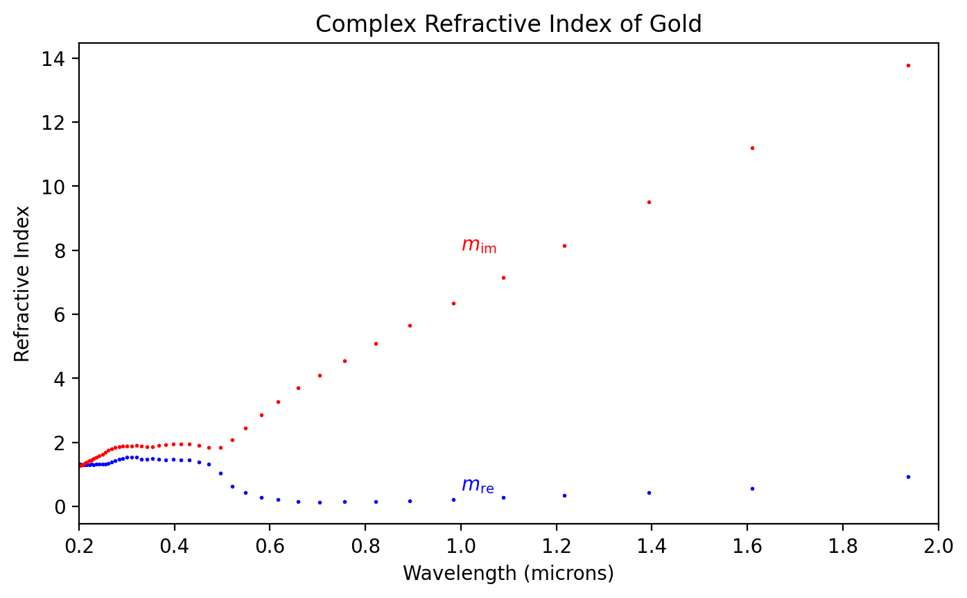
[5]:
# import the Johnson and Christy data for gold
# https://refractiveindex.info/tmp/data/main/Au/Johnson.txt

nname = "data/Johnson.txt"
ref = importlib.resources.files("miepython").joinpath(nname)
au = np.genfromtxt(ref, delimiter="\t")

# data is stacked so need to rearrange
N = len(au) // 2
au_lam = au[1:N, 0]
au_mre = au[1:N, 1]
au_mim = au[N + 1 :, 1]

plt.figure(figsize=(8, 4.5))
plt.scatter(au_lam, au_mre, s=1, color="blue")
plt.scatter(au_lam, au_mim, s=1, color="red")
plt.xlim((0.2, 2))
plt.xlabel("Wavelength (microns)")
plt.ylabel("Refractive Index")
plt.annotate(r"$m_\mathrm{re}$", xy=(1.0, 0.5), color="blue")
plt.annotate(r"$m_\mathrm{im}$", xy=(1.0, 8), color="red")

plt.title("Complex Refractive Index of Gold")

plt.show()
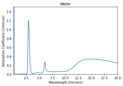
The Absorption Coefficient of Water
[6]:
mua = 4 * np.pi * h2o_mim / h2o_lam

plt.figure(figsize=(8, 4.5))
plt.plot(h2o_lam, mua)
plt.xlim((0.1, 20))
plt.ylim((0, 1.5))
plt.xlabel("Wavelength (microns)")
plt.ylabel("Absorption Coefficient (1/micron)")

plt.title("Water")

plt.show()
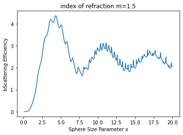
Size Parameters
Size Parameter \(x\)
The sphere size relative to the wavelength is called the size parameter \(x\)
where \(r\) is the radius of the sphere.
[7]:
N = 500
m = 1.5
x = np.linspace(0.1, 20, N)  # also in microns

qext, qsca, qback, g = mie.efficiencies_mx(m, x)

plt.figure(figsize=(8, 4.5))
plt.plot(x, qsca)
plt.xlabel("Sphere Size Parameter x")
plt.ylabel("bScattering Efficiency")
plt.title("index of refraction m=1.5")
plt.show()
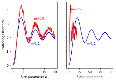
Size Parameter \(\rho\)
The value \(\rho\) is also sometimes used to facilitate comparisons for spheres with different indicies of refraction
Note that when \(m=1.5\) and therefore \(\rho=x\).
As can be seen in the graph below, the scattering for spheres with different indicies of refraction pretty similar when plotted against \(\rho\), but no so obvious when plotted against \(x\)
[8]:
N = 500
m = 1.5
rho = np.linspace(0.1, 20, N)  # also in microns

m = 1.5
x15 = rho / 2 / (m - 1)
qext, sca15, qback, g = mie.efficiencies_mx(m, x15)

m = 1.1
x11 = rho / 2 / (m - 1)
qext, sca11, qback, g = mie.efficiencies_mx(m, x11)

f, (ax1, ax2) = plt.subplots(1, 2, sharey=True, figsize=(8, 4.5))

ax1.plot(rho, sca11, color="blue")
ax1.plot(rho, sca15, color="red")
ax1.set_xlabel(r"Size parameter $\rho$")
ax1.set_ylabel("Scattering Efficiency")
ax1.annotate("m=1.5", xy=(10, 3.3), color="red")
ax1.annotate("m=1.1", xy=(8, 1.5), color="blue")

ax2.plot(x11, sca11, color="blue")
ax2.plot(x15, sca15, color="red")
ax2.set_xlabel(r"Size parameter $x$")
ax2.annotate("m=1.5", xy=(5, 4), color="red")
ax2.annotate("m=1.1", xy=(40, 1.5), color="blue")

plt.show()
Embedded spheres
The short answer is that everything just scales.
Specifically, divide the index of the sphere \(m\) by the index of the surrounding material to get a relative index \(m'\)
The wavelength in the surrounding medium \(\lambda'\) is also altered
Thus, the relative size parameter \(x'\) becomes
Scattering calculations for an embedded sphere uses \(m'\) and \(x'\) instead of \(m\) and \(x\).
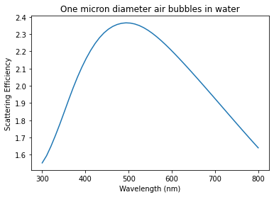
If the spheres are air (\(m=1\)) bubbles in water (\(m=4/3\)), then the relative index of refraction will be about
Here we call mie.efficiencies_mx(m, x) since we have calculated both m and x already.
[12]:
N = 500
mm = 1.0
r = 500  # nm
lambdaa = np.linspace(300, 800, N)  # also in nm

mwater = 4 / 3  # rough approximation
m = mm / mwater
x = 2 * np.pi * r * mwater / lambdaa

qext, qsca, qback, g = mie.efficiencies_mx(m, x)

plt.figure(figsize=(8, 4.5))
plt.plot(lambdaa, qsca)
plt.xlabel("Wavelength (nm)")
plt.ylabel("Scattering Efficiency")
plt.title("One micron diameter air bubbles in water")
plt.show()

or you can just use mie.efficiencies(m_sphere, d_sphere, lambda_vac, n_environ)
[10]:
m_sphere = 1.0
n_water = 4 / 3
d = 1000  # nm
lambda0 = np.linspace(300, 800)  # nm

qext, qsca, qback, g = mie.efficiencies(m_sphere, d, lambda0, n_water)

plt.plot(lambda0, qsca)
plt.xlabel("Wavelength (nm)")
plt.ylabel("Scattering Efficiency")
plt.title("One micron diameter air bubbles in water")
plt.show()
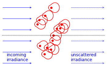
Multiple scatterers
This will eventually turn into a description of the scattering coefficient.
[13]:
m = 1.5
x = np.pi / 3
theta = np.linspace(-180, 180, 1800)
mu = np.cos(theta / 180 * np.pi)
s1, s2 = mie.S1_S2(m, x, mu)
scat = 5 * (abs(s1) ** 2 + abs(s2) ** 2) / 2  # unpolarized scattered light

N = 13
xx = 3.5 * np.random.rand(N, 1) - 1.5
yy = 5 * np.random.rand(N, 1) - 2.5

plt.figure(figsize=(8, 4.5))
plt.scatter(xx, yy, s=40, color="red")
for i in range(N):
    plt.plot(
        scat * np.cos(theta / 180 * np.pi) + xx[i],
        scat * np.sin(theta / 180 * np.pi) + yy[i],
        color="red",
    )

plt.plot([-5, 7], [0, 0], ":k")

plt.annotate("incoming\nirradiance", xy=(-4.5, -2.3), ha="left", color="blue", fontsize=14)
for i in range(6):
    y0 = i - 2.5
    plt.annotate(
        "",
        xy=(-1.5, y0),
        xytext=(-5, y0),
        arrowprops=dict(arrowstyle="->", color="blue"),
    )

plt.annotate("unscattered\nirradiance", xy=(3, -2.3), ha="left", color="blue", fontsize=14)
for i in range(6):
    y0 = i - 2.5
    plt.annotate(
        "",
        xy=(7, y0),
        xytext=(3, y0),
        arrowprops=dict(arrowstyle="->", color="blue", ls=":"),
    )

# plt.annotate('scattered\nspherical\nwave', xy=(0,1.5),ha='left',color='red',fontsize=16)
# plt.annotate('',xy=(2.5,2.5),xytext=(0,0),arrowprops=dict(arrowstyle="->",color='red'))
# plt.annotate(r'$\theta$',xy=(2,0.7),color='red',fontsize=14)
# plt.annotate('',xy=(2,2),xytext=(2.7,0),arrowprops=dict(connectionstyle="arc3,rad=0.2", arrowstyle="<->",color='red'))

plt.xlim(-5, 7)
plt.ylim(-3, 3)
plt.axis("off")
plt.show()
[ ]: