miepython
by Scott Prahl


miepython is a pure Python module to calculate light scattering by
non-absorbing, partially-absorbing, or perfectly conducting spheres. Mie
theory is used, following the procedure described by Wiscombe. This code has
been validated against his results.
This code provides functions for calculating the extinction efficiency, scattering efficiency, backscattering, and scattering asymmetry. Moreover, a set of angles can be given to calculate the scattering at various angles for a sphere.
Heads up!
When comparing different Mie scattering codes, make sure that you’re
aware of the conventions used by each code. miepython makes the
following assumptions
the imaginary part of the complex index of refraction for absorbing spheres is negative.
the scattering phase function is normalized so it equals the single scattering albedo when integrated over 4π steradians by default. As of version 2.3, this can be changed (see the normalization notebook for details).
Using miepython
You can install locally using pip:
pip install miepython
or run this code in the cloud using Google Collaboratory by selecting the Jupyter notebook that interests you.
Script Examples for those that don’t do Jupyter
Simple Dielectric
#!/usr/bin/env python3

"""
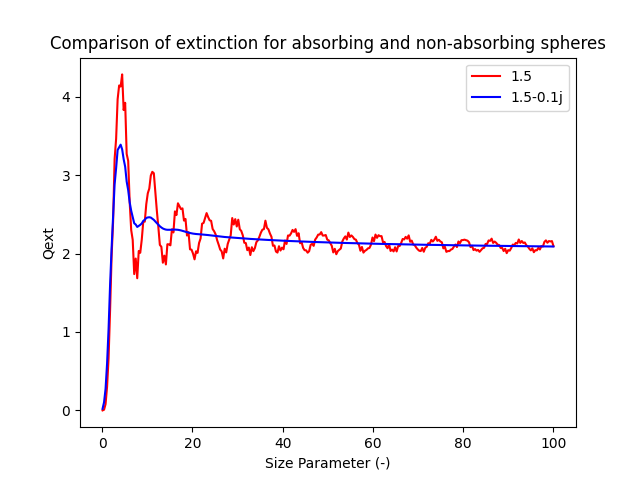
Plot the extinction efficiency as a function of particle size.

This is a comparision of total extinction for non-absorbing and absorbing
spheres.
"""

import numpy as np
import matplotlib.pyplot as plt
import miepython

x = np.linspace(0.1, 100, 300)

# mie() will automatically try to do the right thing

qext, qsca, qback, g = miepython.mie(1.5, x)
plt.plot(x, qext, color='red', label="1.5")

qext, qsca, qback, g = miepython.mie(1.5 - 0.1j, x)
plt.plot(x, qext, color='blue', label="1.5-0.1j")

plt.title("Comparison of extinction for absorbing and non-absorbing spheres")
plt.xlabel("Size Parameter (-)")
plt.ylabel("Qext")
plt.legend()
# plt.show()

Glass Spheres
#!/usr/bin/env python3

"""
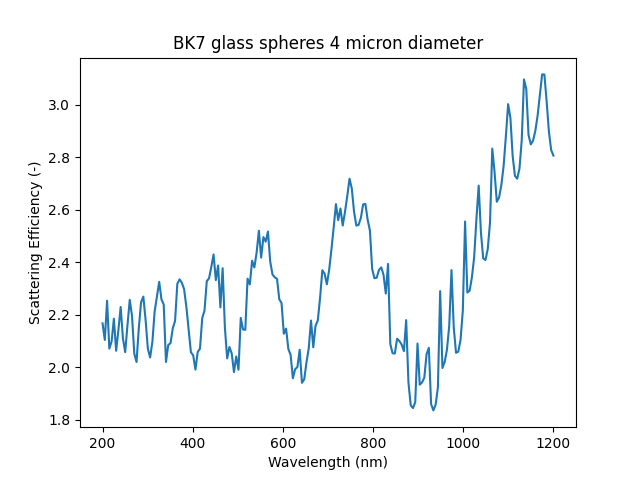
Plot the scattering efficiency for 4 micron glass spheres.

This graph shows scattering as a function of wavelength.
"""

import numpy as np
import matplotlib.pyplot as plt
import miepython

radius = 2                      # in microns
lambda0 = np.linspace(0.2, 1.2, 200)  # also in microns
x = 2 * np.pi * radius / lambda0

# from https://refractiveindex.info/?shelf=glass&book=BK7&page=SCHOTT
m2 = 1 + 1.03961212 / (1 - 0.00600069867 / lambda0**2)
m2 += 0.231792344 / (1 - 0.0200179144 / lambda0**2)
m2 += 1.01046945 / (1 - 103.560653 / lambda0**2)
m = np.sqrt(m2)

qext, qsca, qback, g = miepython.mie(m, x)
plt.plot(lambda0 * 1000, qsca)

plt.title("BK7 glass spheres 4 micron diameter")
plt.xlabel("Wavelength (nm)")
plt.ylabel("Scattering Efficiency (-)")
# plt.show()

Water Droplets
#!/usr/bin/env python3

"""
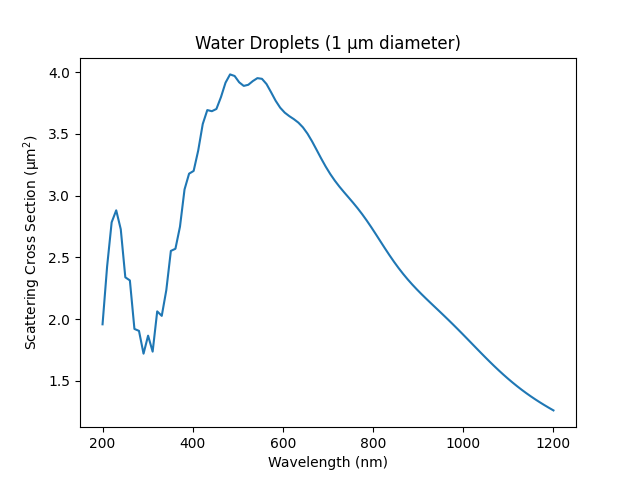
Plot the scattering cross section for 1 micron water droplets.

The plot shows the cross section as a function of wavelength.
"""

import numpy as np
import matplotlib.pyplot as plt
import miepython

num = 100
radius = 0.5                    # in microns
lambda0 = np.linspace(0.2, 1.2, num)  # also in microns
x = 2 * np.pi * radius / lambda0

# from https://refractiveindex.info/?shelf=main&book=H2O&page=Daimon - 24.0C
m2 = 1.0
m2 += 5.666959820E-1 / (1.0 - 5.084151894E-3 / lambda0**2)
m2 += 1.731900098E-1 / (1.0 - 1.818488474E-2 / lambda0**2)
m2 += 2.095951857E-2 / (1.0 - 2.625439472E-2 / lambda0**2)
m2 += 1.125228406E-1 / (1.0 - 1.073842352E1 / lambda0**2)
m = np.sqrt(m2)

qext, qsca, qback, g = miepython.mie(m, x)

plt.plot(lambda0 * 1000, qsca)
plt.title("Water Droplets (1 µm diameter)")
plt.xlabel("Wavelength (nm)")
plt.ylabel("Scattering Cross Section (µm²)")
# plt.show()

Small Gold Spheres
#!/usr/bin/env python3

"""
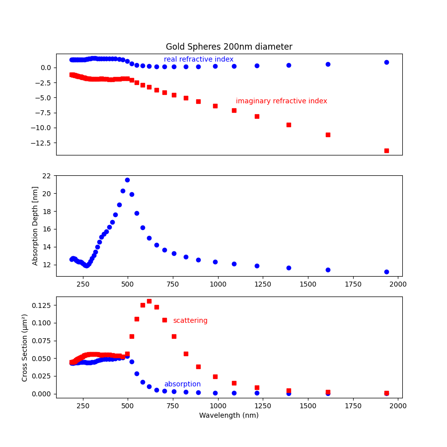
Plot the scattering cross section for 100nm gold spheres.

The resulting graph is as a function of wavelength.
"""

import numpy as np
import matplotlib.pyplot as plt
import miepython

# from https://refractiveindex.info/?shelf = main&book = Au&page = Johnson
# wavelength in microns
ref_lam = np.array([0.1879, 0.1916, 0.1953, 0.1993, 0.2033, 0.2073, 0.2119, 0.2164,
                    0.2214, 0.2262, 0.2313, 0.2371, 0.2426, 0.2490, 0.2551, 0.2616,
                    0.2689, 0.2761, 0.2844, 0.2924, 0.3009, 0.3107, 0.3204, 0.3315,
                    0.3425, 0.3542, 0.3679, 0.3815, 0.3974, 0.4133, 0.4305, 0.4509,
                    0.4714, 0.4959, 0.5209, 0.5486, 0.5821, 0.6168, 0.6595, 0.7045,
                    0.7560, 0.8211, 0.8920, 0.9840, 1.0880, 1.2160, 1.3930, 1.6100, 1.9370])

ref_n = np.array([1.28, 1.32, 1.34, 1.33, 1.33, 1.30, 1.30, 1.30, 1.30, 1.31, 1.30,
                  1.32, 1.32, 1.33, 1.33, 1.35, 1.38, 1.43, 1.47, 1.49, 1.53, 1.53,
                  1.54, 1.48, 1.48, 1.50, 1.48, 1.46, 1.47, 1.46, 1.45, 1.38, 1.31,
                  1.04, 0.62, 0.43, 0.29, 0.21, 0.14, 0.13, 0.14, 0.16, 0.17, 0.22,
                  0.27, 0.35, 0.43, 0.56, 0.92])

ref_k = np.array([1.188, 1.203, 1.226, 1.251, 1.277, 1.304, 1.350, 1.387, 1.427,
                  1.460, 1.497, 1.536, 1.577, 1.631, 1.688, 1.749, 1.803, 1.847,
                  1.869, 1.878, 1.889, 1.893, 1.898, 1.883, 1.871, 1.866, 1.895,
                  1.933, 1.952, 1.958, 1.948, 1.914, 1.849, 1.833, 2.081, 2.455,
                  2.863, 3.272, 3.697, 4.103, 4.542, 5.083, 5.663, 6.350, 7.150,
                  8.145, 9.519, 11.21, 13.78])

radius = 0.1                    # in microns
m = ref_n - 1.0j * ref_k
x = 2 * np.pi * radius / ref_lam
cross_section_area = np.pi * radius ** 2
mu_a = 4 * np.pi * ref_k / ref_lam    # nm
qext, qsca, qback, g = miepython.mie(m, x)

sca_cross_section = qsca * cross_section_area
abs_cross_section = (qext - qsca) * cross_section_area

plt.subplots(3, 1, figsize=(9, 9))
plt.subplot(311)
plt.plot(ref_lam * 1000, ref_n, 'ob')
plt.plot(ref_lam * 1000, -ref_k, 'sr')
plt.title("Gold Spheres 200nm diameter")
plt.text(700, 1, "real refractive index", color='blue')
plt.text(1100, -6, "imaginary refractive index", color='red')

plt.subplot(312)
plt.plot(ref_lam * 1000, 1000 / mu_a, 'ob')
plt.ylabel("Absorption Depth [nm]")

plt.subplot(313)
plt.plot(ref_lam * 1000, abs_cross_section, 'ob')
plt.plot(ref_lam * 1000, sca_cross_section, 'sr')
plt.xlabel("Wavelength (nm)")
plt.ylabel("Cross Section (µm²)")
plt.text(700, 0.01, "absorption", color='blue')
plt.text(750, 0.1, "scattering", color='red')
#plt.savefig("04_plot.png")
# plt.show()
