Mie Scattering and Fog
Scott Prahl
Feb 2025
Clouds are one of the big reasons that Mie scattering is useful. This notebook covers the basics of log normal distributions and shows a few calculations using miepython.
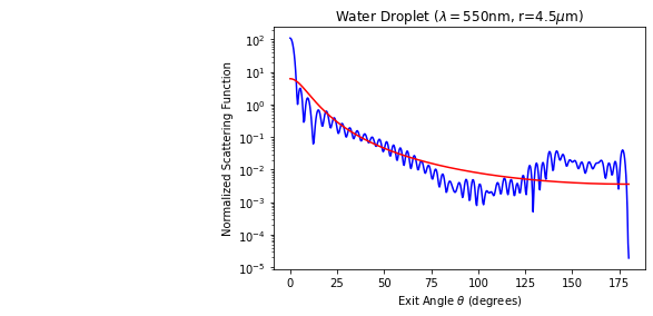
One conclusion of this notebook is that for relatively large water droplets, the Henyey-Greenstein phase function is a poor approximation for the forward scattered light.
[1]:
%config InlineBackend.figure_format = 'retina'

import os
import sys
import numpy as np
import matplotlib.pyplot as plt
from scipy import stats  # needed for lognormal distribution

if sys.platform == "emscripten":
    import piplite

    await piplite.install("miepython", deps=False)
    os.environ["MIEPYTHON_USE_JIT"] = "0"  # jupyterlite cannot use numba

import miepython as mie
Fog data
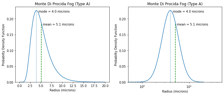
Scattering depends on the size distribution of droplets as well as the droplet density. In general, the distributions have been modelled as log-normal or as a gamma function. This notebook focuses on the log-normal distribution.
Fog data from Podzimek, “Droplet Concentration and Size Distribution in Haze and Fog”, Studia geoph. et geod. 41 (1997).
For the first trick I’ll show that the log-normal distribution is just a plain old normal distribution but with a logarthmic horizontal axis. Also note that the mean droplet size and the most common size (mode) differ.
[2]:
fogtype = "Monte Di Procida Fog (Type A)"  # most common fog
r_g = 4.69  # in microns
sigma_g = 1.504  # in microns

shape = np.log(sigma_g)
mode = np.exp(np.log(r_g) - np.log(sigma_g) ** 2)
mean = np.exp(np.log(r_g) + np.log(sigma_g) ** 2 / 2)

num = 100
r = np.linspace(0.1, 20, num)  # values for x-axis

pdf = stats.lognorm.pdf(r, shape, scale=r_g)  # probability distribution

plt.figure(figsize=(12, 4.5))
# Figure on linear scale
plt.subplot(121)

plt.plot(r, pdf)
plt.vlines(mode, 0, pdf.max(), linestyle=":", label="Mode")
plt.vlines(
    mean,
    0,
    stats.lognorm.pdf(mean, shape, scale=r_g),
    linestyle="--",
    color="green",
    label="Mean",
)
plt.annotate("mode = 4.0 microns", xy=(4.5, 0.22))
plt.annotate("mean = 5.1 microns", xy=(5.5, 0.18))

plt.ylim(ymin=0)
plt.xlabel("Radius (microns)")
plt.ylabel("Probabilty Density Function")
plt.title(fogtype)

plt.subplot(122)
plt.semilogx(r, pdf)

plt.vlines(mode, 0, pdf.max(), linestyle=":", label="Mode")
plt.vlines(
    mean,
    0,
    stats.lognorm.pdf(mean, shape, scale=r_g),
    linestyle="--",
    color="green",
    label="Mean",
)
plt.annotate("mode = 4.0 microns", xy=(4.5, 0.22))
plt.annotate("mean = 5.1 microns", xy=(5.5, 0.18))

plt.ylim(ymin=0)
plt.xlabel("Radius (microns)")
plt.xlim(0.5, 50)
plt.ylabel("Probabilty Density Function")
plt.title(fogtype)
plt.show()

Scattering Asymmetry from Fog
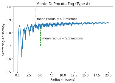
So the average cosine of the scattering phase function is often called the scattering asymmetry or just the scattering anisotropy. The value lies between -1 (completely back scattering) and +1 (total forward scattering). For these fog values, the scattering is pretty strongly forward scattering.
[3]:
num = 400  # number of droplet sizes to process

# distribution of droplet sizes in fog
fogtype = "Monte Di Procida Fog (Type A)"
r_g = 4.69  # in microns
sigma_g = 1.504  # in microns
shape = np.log(sigma_g)
mode = np.exp(np.log(r_g) - np.log(sigma_g) ** 2)
mean = np.exp(np.log(r_g) + np.log(sigma_g) ** 2 / 2)

r = np.linspace(0.1, 20, num)  # values for x-axis
pdf = stats.lognorm.pdf(r, shape, scale=r_g)  # probability distribution

# scattering cross section for each droplet size
lambdaa = 0.550  # in microns
m = 1.33
x = 2 * np.pi * r / lambdaa

qext, qsca, qback, g = mie.efficiencies_mx(m, x)

plt.figure(figsize=(8, 4.5))
plt.plot(r, g)
plt.ylim(0.5, 1.0)
plt.xlabel("Radius (microns)")
plt.ylabel("Scattering Anisotropy")
plt.title(fogtype)
plt.vlines(mode, 0.85, 1, linestyle=":", label="Mode")
plt.vlines(mean, 0.7, 0.85, linestyle="--", color="green", label="Mean")
plt.annotate("mode radius = 4.0 microns", xy=(4.3, 0.9))
plt.annotate("mean radius = 5.1 microns", xy=(5.5, 0.75))

plt.show()
Scattering as a function of angle
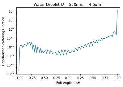
Let’s take a closer look at scattering between the mode and mean radius.
[4]:
num = 100  # number of angles

# scattering cross section for each droplet size
lambdaa = 0.550  # in microns
m = 1.33
r = 4.5  # in microns

x = 2 * np.pi * r / lambdaa
mu = np.linspace(-1, 1, num)
s1, s2 = mie.S1_S2(m, x, mu)
scatter = 0.5 * (abs(s1) ** 2 + abs(s2) ** 2)

plt.figure(figsize=(8, 4.5))
plt.plot(mu, scatter)
plt.yscale("log")
plt.xlim(-1.05, 1.05)
# plt.ylim(ymin=0.8)
plt.xlabel(r"Exit Angle $\cos\theta$")
plt.ylabel("Unpolarized Scattering Function")
plt.title(r"Water Droplet ($\lambda=550$nm, r=4.5$\mu$m)")

plt.show()
The graph above does not really do justice to how strongly forward scattering the water droplets are! Here is a close up of four droplet radii (1,5,10,20) microns. The most common fog size (5 micron) has a FWHM of 2.5°
[5]:
num = 100  # number of angles

# scattering cross section for each droplet size
lambdaa = 0.550
m = 1.33
r = 4.5
theta = np.linspace(0, 5, num)
mu = np.cos(theta * np.pi / 180)

r = np.array([1, 5, 10, 20])
kolor = np.array(["red", "green", "blue", "black"])
for i in range(4):
    x = 2 * np.pi * r[i] / lambdaa
    s1, s2 = mie.S1_S2(m, x, mu)
    scatter = 0.5 * (abs(s1) ** 2 + abs(s2) ** 2)
    plt.plot(theta, scatter / scatter[0], color=kolor[i])
    plt.plot(-theta, scatter / scatter[0], color=kolor[i])

plt.annotate("r=%.0f" % r[0], xy=(3.8, 0.84), color=kolor[0])
plt.annotate("r=%.0f" % r[1], xy=(1.8, 0.5), color=kolor[1])
plt.annotate("r=%.0f" % r[2], xy=(1, 0.3), color=kolor[2])
plt.annotate("r=%.0f" % r[3], xy=(-0.1, 0.0), color=kolor[3])

# plt.yscale('log')
# plt.ylim(ymin=0.8)
plt.xlabel(r"Exit Angle $\theta$ (degrees)")
plt.ylabel("Normalized Scattering Function")
plt.title(r"Water Droplet ($\lambda=550$nm, r=4.5$\mu$m)")

plt.show()
Henyey-Greenstein Phase Function
How does the Mie scattering for a 5 micron droplet radius compare with Henyey-Greenstein?
First, need to make sure both scattering functions are normalized to the same overall value. If we integrate over all \(4\pi\) steradians
This is can be approximated as
when all the scattering angles are equally spaced in \(\cos\theta\).
The integral over all angles for Mie scattering is not 1. Instead it is \(\pi x^2 Q_\mathrm{sca}\) as we see below.
[6]:
def hg(g, costheta):
    """Henyey-Greenstein scattering phase function."""
    return (1 / 4 / np.pi) * (1 - g**2) / (1 + g**2 - 2 * g * costheta) ** 1.5


num = 1000  # increase number of angles to improve integration
r = 0.45  # in microns
lambdaa = 0.550  # in microns
m = 1.33

x = 2 * np.pi * r / lambdaa
k = 2 * np.pi / lambdaa
qext, qsca, qback, g = mie.efficiencies_mx(m, x)

mu = np.linspace(-1, 1, num)
s1, s2 = mie.S1_S2(m, x, mu)
miescatter = 0.5 * (abs(s1) ** 2 + abs(s2) ** 2)
hgscatter = hg(g, mu)

delta_mu = mu[1] - mu[0]
total = 2 * np.pi * delta_mu * np.sum(miescatter)

print("mie integral= ", total)

total = 2 * np.pi * delta_mu * np.sum(hgscatter)
print("hg integral= ", total)
mie integral=  1.0137512825791524
hg integral=  1.0405143428517407
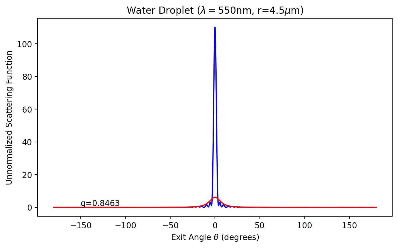
Now we can see how bad the approximation is when using the Henyey-Greenstein function. Here is a log plot
[7]:
num = 500
r = 4.5
lambdaa = 0.550
m = 1.33
x = 2 * np.pi * r / lambdaa

theta = np.linspace(0, 180, num)
mu = np.cos(theta * np.pi / 180)

s1, s2 = mie.S1_S2(m, x, mu)
miescatter = 0.5 * (abs(s1) ** 2 + abs(s2) ** 2)

plt.figure(figsize=(8, 4.5))
plt.plot(theta, miescatter, color="blue")
plt.plot(theta, hg(g, mu), color="red")
plt.yscale("log")
plt.xlabel(r"Exit Angle $\theta$ (degrees)")
plt.ylabel("Normalized Scattering Function")
plt.title(r"Water Droplet ($\lambda=550$nm, r=4.5$\mu$m)")
plt.annotate("g=%.4f" % g, xy=(-150, 0.9))
plt.show()

Here is some naive scaling on a non-log scale
[8]:
num = 500  # number of angles
r = 4.5  # microns
lambdaa = 0.550  # microns
m = 1.33

x = 2 * np.pi * r / lambdaa
theta = np.linspace(0, 180, num)
mu = np.cos(theta * np.pi / 180)

s1, s2 = mie.S1_S2(m, x, mu)
miescatter = 0.5 * (abs(s1) ** 2 + abs(s2) ** 2)
hgscatter = hg(g, mu)

plt.figure(figsize=(8, 4.5))
plt.plot(theta, miescatter / miescatter[0], color="blue")
plt.plot(-theta, miescatter / miescatter[0], color="blue")
plt.plot(theta, hg(g, mu) / hg(g, 1), color="red")
plt.plot(-theta, hg(g, mu) / hg(g, 1), color="red")
plt.xlabel(r"Exit Angle $\theta$ (degrees)")
plt.ylabel("Normalized Scattering Function")
plt.title(r"Water Droplet ($\lambda=550$nm, r=4.5$\mu$m)")
plt.annotate("g=%.4f" % g, xy=(-150, 0.9))
plt.show()
[9]:
plt.plot(theta, miescatter, color="blue")
plt.plot(-theta, miescatter, color="blue")
plt.plot(theta, hg(g, mu), color="red")
plt.plot(-theta, hg(g, mu), color="red")
plt.xlabel(r"Exit Angle $\theta$ (degrees)")
plt.ylabel("Unnormalized Scattering Function")
plt.title(r"Water Droplet ($\lambda=550$nm, r=4.5$\mu$m)")
plt.annotate("g=%.4f" % g, xy=(-150, 0.9))
plt.show()

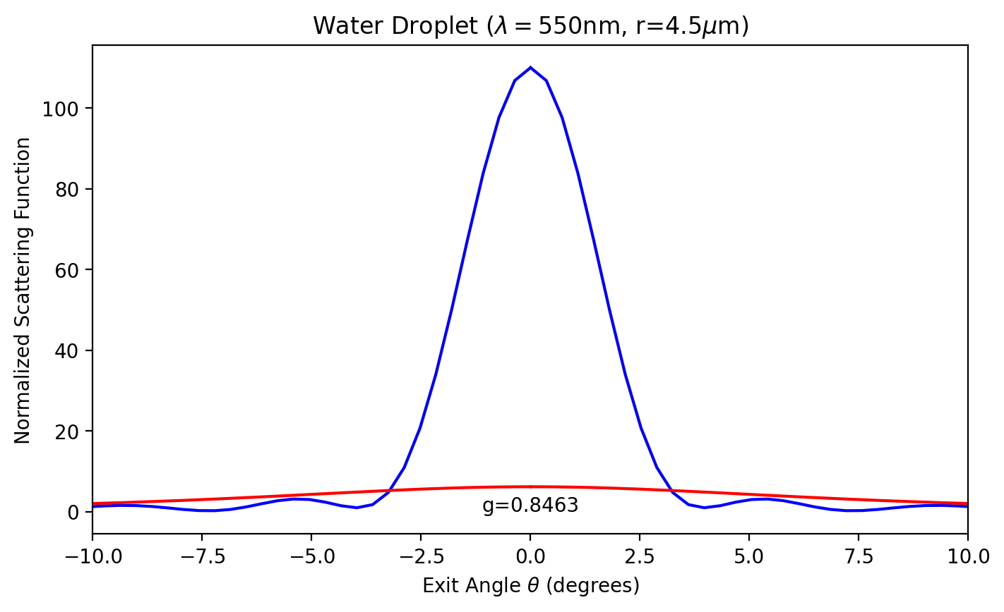
[10]:
plt.plot(theta, miescatter, color="blue")
plt.plot(-theta, miescatter, color="blue")
plt.plot(theta, hg(g, mu), color="red")
plt.plot(-theta, hg(g, mu), color="red")
plt.xlabel(r"Exit Angle $\theta$ (degrees)")
plt.ylabel("Normalized Scattering Function")
plt.title(r"Water Droplet ($\lambda=550$nm, r=4.5$\mu$m)")
plt.text(0.0, 0, "g=%.4f" % g, ha="center")
plt.xlim([-10, 10])
plt.show()
[11]:
num = 100

# distribution of droplet sizes in fog
r = np.linspace(0.1, 20, num)  # values for x-axis
pdf = stats.lognorm.pdf(r, shape, scale=r_g)  # probability distribution

# scattering cross section for each droplet size
lambdaa = 0.550
m = 1.33
x = 2 * np.pi * r / lambdaa

qext, qsca, qback, g = mie.efficiencies_mx(m, x)
cross_section = qsca * np.pi * r**2 * (1 - g)

# weighted average of the cross_sections
mean_cross = 0
mean_r = 0
for i in range(num):
    mean_cross += cross_section[i] * pdf[i]
    mean_r += cross_section[i] * pdf[i] * r[i]
mean_r /= mean_cross
mean_cross /= num

plt.plot(r, cross_section * pdf)
# plt.plot(r,pdf*100)

plt.plot((mean_r, mean_r), (0, 40))
plt.plot((0, 20), (mean_cross, mean_cross))

plt.ylim(0, 6)
plt.xlabel("Radius (microns)")
plt.ylabel("Weighted Scattering Cross-Section (um2)")
plt.annotate("mean cross section =%.2f" % mean_cross, xy=(11, mean_cross + 0.1))
plt.annotate("mean size =%.2f" % mean_r, xy=(mean_r, 0.2))

plt.title(fogtype)
plt.show()
[ ]: