Rayleigh Scattering

Scott Prahl

March 2025

[1]:

%config InlineBackend.figure_format = 'retina'

import os
import sys
import numpy as np
import matplotlib.pyplot as plt

if sys.platform == "emscripten":
    import piplite

    await piplite.install("miepython", deps=False)
    os.environ["MIEPYTHON_USE_JIT"] = "0"  # jupyterlite cannot use numba

import miepython as mie
from miepython import rayleigh as ray

Goals for this notebook:

Plot Rayleigh scattering
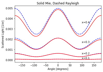
Compare total scattering between Rayleigh and Mie
Compare scattering functions for unpolarized light
Compare polarized results.

Rayleigh Scattering Functions

Mie scattering describes the special case of the interaction of light passing through a non-absorbing medium with a single embedded spherical object. The sphere itself can be non-absorbing, moderately absorbing, or perfectly absorbing.

Rayleigh scattering is a simple closed-form solution for the scattering from small spheres.

The Rayleigh scattering phase function

Rayleigh scattering describes the elastic scattering of light by spheres that are much smaller than the wavelength of light. The intensity \(I\) of the scattered radiation is given by

\[I=I_{0}\left(\frac {1+\cos ^{2}\theta }{2R^{2}}\right) \left(\frac {2\pi }{\lambda }\right)^{4} \left(\frac {n^{2}-1}{n^{2}+2}\right)^{2} \left(\frac {d}{2}\right)^{6}\]

where \(I_0\) is the light intensity before the interaction with the particle, \(R\) is the distance between the particle and the observer, \(\theta\) is the scattering angle, \(n\) is the refractive index of the particle, and \(d\) is the diameter of the particle.

\[x = \frac{\pi d}{\lambda} \qquad \rho=\frac{R}{\lambda}\]

and thus

\[I=\frac{I_0}{8\pi^2\rho^2} \left(\frac{n^2-1}{n^2+2}\right)^{2} x^{4}(1+\cos^2\theta)\]

Compare Efficiencies with Mie Code

[2]:

for x in [0.1, 0.2, 0.3, 0.4]:

    m = 1.5 - 1j
    theta = np.linspace(-180, 180, 180)
    mu = np.cos(theta * np.pi / 180)

    rscat = ray.i_unpolarized(m, x, mu)
    mscat = mie.i_unpolarized(m, x, mu)
    plt.plot(theta, rscat, "--b")
    plt.plot(theta, mscat, "r")
    plt.annotate("x=%.1f   " % x, (theta[-20], mscat[-20]), ha="right", va="bottom")

plt.xlim(-180, 180)
plt.xlabel("Angle [degrees]")
plt.ylabel("Scattered Light [1/sr]")
plt.title("Solid Mie, Dashed Rayleigh")
plt.show()

Polar plots for fun

[3]:

m = 1.5
x = 0.1
theta = np.linspace(-180, 180, 180)
mu = np.cos(theta / 180 * np.pi)
unp = ray.i_unpolarized(m, x, mu)
s1, s2 = ray.S1_S2(m, x, mu)
par = abs(s1) ** 2
per = abs(s2) ** 2

fig, ax = plt.subplots(1, 2, figsize=(12, 5))
ax = plt.subplot(121, projection="polar")
ax.plot(theta / 180 * np.pi, unp)
ax.plot(theta / 180 * np.pi, par)
ax.plot(theta / 180 * np.pi, per)

ax.set_rticks([0.05, 0.1, 0.15])

plt.subplot(122)
# plt.plot(theta,scat)
plt.plot(theta, unp)
plt.plot(theta, par)
plt.plot(theta, per)

plt.xlabel("Exit Angle [degrees]")
plt.ylabel("Unpolarized Scattered light [1/sr]")
plt.title("m=1.5, x = %.2f" % x)

plt.ylim(0.00, 0.2)
plt.xlim(0, 180)

plt.show()

Compare Rayleigh and Mie efficiencies

[4]:

m = 1.5
x = 0.1
qext, qsca, qback, g = mie.efficiencies_mx(m, x)
rext, rsca, rback, rg = ray.efficiencies_mx(m, x)

print("Qext        Qsca        Qback       g")
print("%.5e %.5e %.5e %.5f Mie" % (qext, qsca, qback, g))
print("%.5e %.5e %.5e %.5f Rayleigh" % (rext, rsca, rback, rg))

Qext        Qsca        Qback       g
2.30841e-05 2.30841e-05 3.44629e-05 0.00198 Mie
2.30681e-05 2.30681e-05 3.46021e-05 0.00000 Rayleigh

Compare scattering amplitudes S1 and S2

[5]:

m = 1.5
x = 0.1
theta = np.linspace(-180, 180, 19)
mu = np.cos(np.deg2rad(theta))

s1, s2 = mie.S1_S2(m, x, mu)
rs1, rs2 = ray.S1_S2(m, x, mu)

# the real part of the Rayleigh scattering is always zero

print("          Mie       Rayleigh | Mie      Rayleigh")
print("  angle | S1.imag    S1.imag | S2.imag  S2.imag")
print("------------------------------------------------")
for i, angle in enumerate(theta):
    print("%7.2f | %8.5f  %8.5f | %8.5f %8.5f " % (angle, s1[i].imag, rs1[i].imag, s2[i].imag, rs2[i].imag))

          Mie       Rayleigh | Mie      Rayleigh
  angle | S1.imag    S1.imag | S2.imag  S2.imag
------------------------------------------------
-180.00 |  0.34468   0.34562 | -0.34468 -0.34562
-160.00 |  0.34473   0.34562 | -0.32392 -0.32477
-140.00 |  0.34487   0.34562 | -0.26412 -0.26476
-120.00 |  0.34509   0.34562 | -0.17242 -0.17281
-100.00 |  0.34535   0.34562 | -0.05981 -0.06002
 -80.00 |  0.34563   0.34562 |  0.06018  0.06002
 -60.00 |  0.34590   0.34562 |  0.17307  0.17281
 -40.00 |  0.34612   0.34562 |  0.26521  0.26476
 -20.00 |  0.34626   0.34562 |  0.32540  0.32477
   0.00 |  0.34631   0.34562 |  0.34631  0.34562
  20.00 |  0.34626   0.34562 |  0.32540  0.32477
  40.00 |  0.34612   0.34562 |  0.26521  0.26476
  60.00 |  0.34590   0.34562 |  0.17307  0.17281
  80.00 |  0.34563   0.34562 |  0.06018  0.06002
 100.00 |  0.34535   0.34562 | -0.05981 -0.06002
 120.00 |  0.34509   0.34562 | -0.17242 -0.17281
 140.00 |  0.34487   0.34562 | -0.26412 -0.26476
 160.00 |  0.34473   0.34562 | -0.32392 -0.32477
 180.00 |  0.34468   0.34562 | -0.34468 -0.34562

[ ]: